Projects-Portfolio

Solar System Positions · 1900–2100

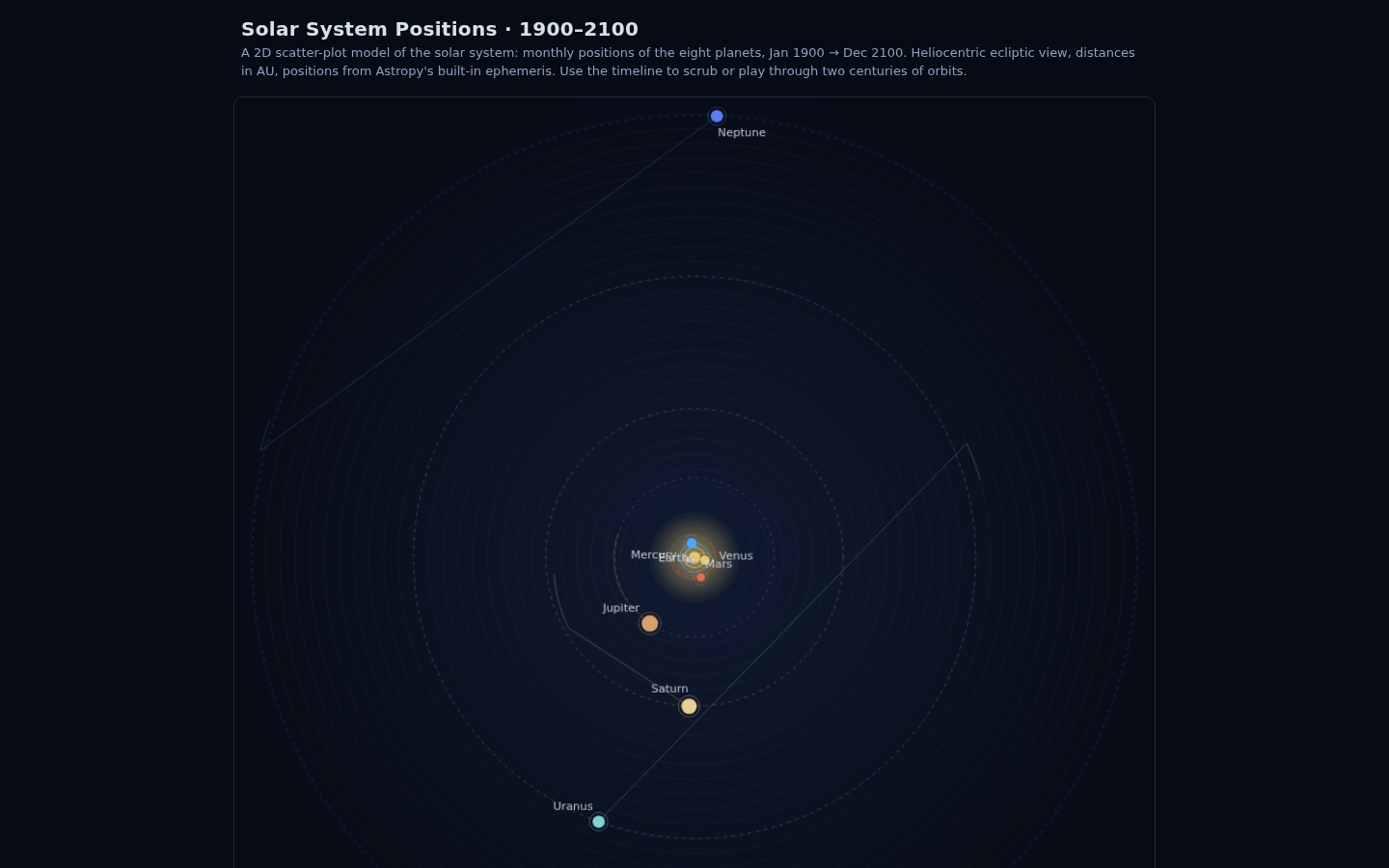
An interactive 2D scatter-plot model of the solar system: the position of every planet, plotted for every month from January 1900 to December 2100, with a controllable timeline. 2412 monthly frames, 8 planets, one self-contained HTML file.

Problem

Textbook orbit diagrams are static snapshots. When you want to feel how the planets move — Mercury lapping Earth, Jupiter’s slow twelve-year circuit, Neptune barely creeping along — you need an animation over a long baseline. Most interactive solar-system demos fetch live data or cover a few years. This one shows the full 1900–2100 range with honest, reproducible ephemeris positions, and it lives entirely in the repository: no server, no CDN, no downloads at view time.

Approach

Compute positions with Astropy. For the first day of every month, each planet’s barycentric ICRS position is differenced against the Sun’s and rotated into the mean ecliptic plane → heliocentric ecliptic (x, y) in AU, the classic top-down “map” of the solar system. The default ephemeris is Astropy’s built-in (ERFA) planetary model: fully offline, deterministic, and accurate to well beyond what a scatter plot needs. (An optional --ephemeris jpl --include-pluto flag produces arcsecond-grade JPL DE440s positions including the dwarf planet, at the cost of a one-time ephemeris download.)
Generate the data: data/positions.csv — 19,296 rows (2,412 months × 8 planets), rounded to 1e-6 AU (~150 km), committed in full because it is small and reproducible.
Build the viewer: viewer.html — a single self-contained file. A Canvas scatter plot with the Sun at the origin, planet dots on current-distance orbit guides, trails, a hover readout (exact AU from the Sun), and a timeline you can scrub with a slider, step with the arrow keys, or play back at 1–120 months/second. Log-scale toggle keeps the inner planets visible next to Neptune’s 30 AU. All 2,412 frames are embedded in the file — it works from GitHub Pages, any static host, or by double-clicking locally.

Results

Metric	Value
Frames	2,412 (Jan 1900 → Dec 2100, monthly)
Bodies	Mercury, Venus, Earth, Mars, Jupiter, Saturn, Uranus, Neptune
Data rows	19,296
Data size	~700 KB CSV (committed)
Viewer size	~550 KB single HTML file
Ephemeris	Astropy built-in (ERFA) — offline, deterministic
Precision	1e-6 AU (~150 km)
Tests	hermetic: shape, finiteness, orbit ordering, golden Astropy checks

View the interactive chart: https://richard-ws.github.io/Projects-Portfolio/experiments/solar-system-positions/viewer.html (or open viewer.html locally — it is fully self-contained).

Validation highlights (all enforced by the test suite):

Every one of the 2,412 frames has exactly the 8 planets, all coordinates finite.
Radial ordering never violates Mercury < Venus < … < Neptune at any month over 200 years.
Earth stays within 0.95–1.05 AU of the Sun for every frame.
A golden test recomputes six (date, planet) pairs directly with Astropy and confirms the committed CSV matches to 5e-5 AU.
An orientation check pins Earth near ecliptic longitude 180° at the March 2000 equinox (x < −0.9), proving the ICRS→ecliptic rotation sign is correct — a mirrored solar system would fail this instantly.

Quick start

python -m venv .venv
.venv/bin/pip install -e ".[dev]"

# regenerate the full dataset (offline, ~seconds):
.venv/bin/python scripts/generate_positions.py -c configs/example.yaml

# rebuild the viewer from the CSV:
.venv/bin/python scripts/build_viewer.py -c configs/example.yaml

# run the hermetic test suite:
.venv/bin/pytest

Optional JPL + Pluto variant (arcsecond-grade, needs one-time download):

.venv/bin/python scripts/generate_positions.py -c configs/example.yaml \
    --ephemeris jpl --include-pluto
.venv/bin/python scripts/build_viewer.py -c configs/example.yaml

Caveats

Accuracy: the built-in ephemeris is an analytic planetary model (ERFA), accurate to arcsecond/arcminute level over 1900–2100. Invisible at scatter-plot scale; use --ephemeris jpl if you need JPL-grade numbers.
2D projection: positions are projected onto the ecliptic plane (z ignored). Inclinations of up to ~7° (Mercury) mean the plotted distance is a slight underestimate of the true 3D distance.
No Pluto by default: the built-in ephemeris covers the eight planets only; Pluto needs the JPL ephemeris (flag above).
One machine, one range: results describe the computed dataset; regeneration is deterministic given the same Astropy version.

Layout

solar-system-positions/
├── configs/example.yaml      # range, bodies, ephemeris, output paths
├── src/solarpositions/
│   ├── config.py             # YAML config with numeric coercion
│   ├── positions.py          # Astropy ephemeris → ecliptic (x, y)
│   └── build.py              # CSV → embedded JSON → viewer.html
├── scripts/
│   ├── generate_positions.py # data/positions.csv
│   └── build_viewer.py       # viewer.html
├── templates/viewer_template.html  # the Canvas app (placeholder for data)
├── data/positions.csv        # committed generated data (19,296 rows)
├── viewer.html               # committed self-contained viewer
└── tests/                    # 20 hermetic tests

This site is open source. Improve this page.